Examples

Five worked examples in order of increasing complexity. Each includes a code block, expected output, and a generated image.

Example 1 – Your First Optimization

Build a 2x2 grid, optimize at a single time step, and inspect the result.

import numpy as np
from chiller_sim import Simulator

sim = (
    Simulator()
    .with_grid(rows=2, cols=2, spacing_m=10.0, base_cop=4.0, max_cooling_kw=500.0)
    .with_wind(speed_m_per_s=5.0, angle_deg=0.0)
    .with_ambient_temp(temp_k=298.15)
    .with_load_fn(lambda t: 800.0)
    .build()
)

result = sim.optimize(time_hours=0.0)

print(f"Active mask:     {result.active_mask}")
print(f"COP per chiller: {np.round(result.cop_array, 2)}")
print(f"Total work:      {result.total_work_kw:.2f} kW")

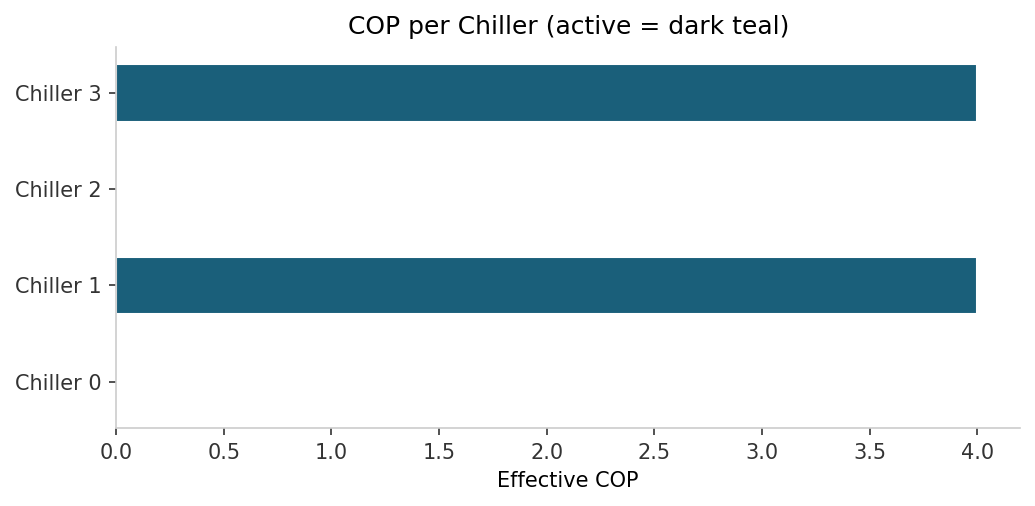
Horizontal bar chart of COP for each chiller – active bars in dark teal, inactive bars in light grey.

Example 2 – Thermal Interference

A 1x4 row of chillers with wind blowing along the row. Downwind chillers run hotter because they sit in the exhaust plume of upwind neighbours.

import numpy as np
from chiller_sim import Simulator

sim = (
    Simulator()
    .with_grid(rows=1, cols=4, spacing_m=10.0, base_cop=4.0, max_cooling_kw=500.0)
    .with_wind(speed_m_per_s=5.0, angle_deg=0.0)
    .with_ambient_temp(temp_k=298.15)
    .with_load_fn(lambda t: 1000.0)
    .build()
)

result = sim.optimize(time_hours=0.0)

print("Inlet temperature rise at each position:")
for i, rise in enumerate(result.temp_rise_array):
    print(f"  Chiller {i}: {rise:.3f} K")

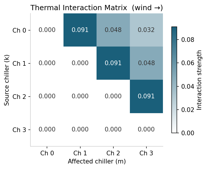
Heatmap of the 4x4 interaction matrix – dark teal for high interaction, white for zero.

Example 3 – Capacity, Aging, and the Feasibility Gate

Two simulations at the same load: a brand-new fleet vs. an aged fleet. Aged chillers have lower effective capacity, so more must activate to meet the load.

import numpy as np
from chiller_sim import Simulator

load_kw = 800.0

# New fleet
sim_new = (
    Simulator()
    .with_grid(rows=2, cols=2, spacing_m=10.0, base_cop=4.0,
               max_cooling_kw=500.0, ages_years=np.zeros(4))
    .with_wind(speed_m_per_s=5.0, angle_deg=0.0)
    .with_ambient_temp(temp_k=298.15)
    .with_load_fn(lambda t: load_kw)
    .build()
)

# Aged fleet (20 years old)
sim_aged = (
    Simulator()
    .with_grid(rows=2, cols=2, spacing_m=10.0, base_cop=4.0,
               max_cooling_kw=500.0, ages_years=np.full(4, 20.0))
    .with_wind(speed_m_per_s=5.0, angle_deg=0.0)
    .with_ambient_temp(temp_k=298.15)
    .with_load_fn(lambda t: load_kw)
    .build()
)

r_new = sim_new.optimize(time_hours=0.0)
r_aged = sim_aged.optimize(time_hours=0.0)

print(f"New fleet:  {r_new.active_mask.sum()} active, {r_new.total_work_kw:.1f} kW")
print(f"Aged fleet: {r_aged.active_mask.sum()} active, {r_aged.total_work_kw:.1f} kW")

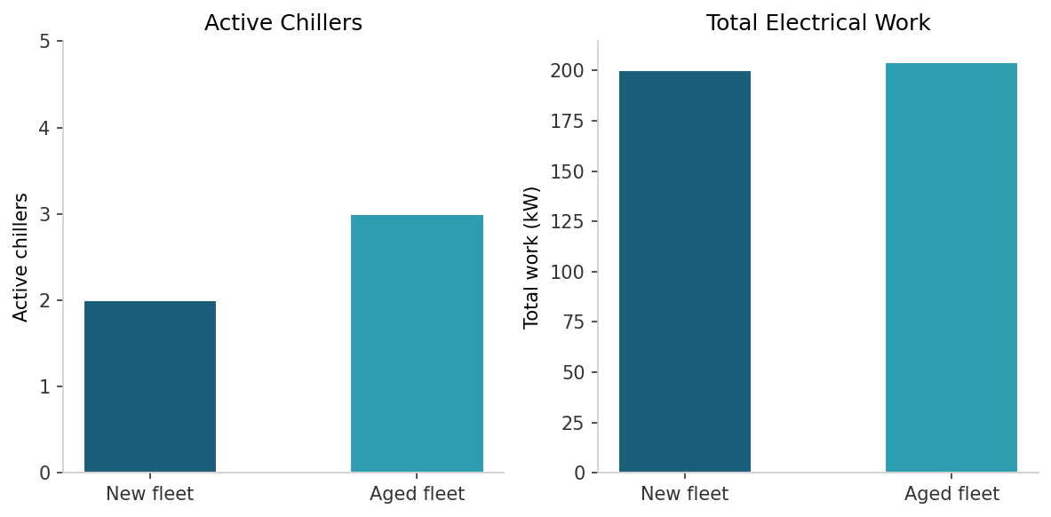
Grouped bar chart – two groups (new / aged), bars showing number of active chillers and total work side by side.

Example 4 – Streaming a 24-Hour Load Profile

Sinusoidal load function (300–800 kW, 24 h period) fed to stream() with a 1 h time step.

import math
from chiller_sim import Simulator

sim = (
    Simulator()
    .with_grid(rows=2, cols=4, spacing_m=10.0, base_cop=4.0, max_cooling_kw=500.0)
    .with_wind(speed_m_per_s=5.0, angle_deg=0.0)
    .with_ambient_temp(temp_k=298.15)
    .with_load_fn(lambda t: 550.0 + 250.0 * math.sin(2 * math.pi * t / 24))
    .build()
)

for result in sim.stream(duration_hours=24.0, time_step_hours=1.0):
    n = result.active_mask.sum()
    print(f"t={result.time_hours:5.1f}h  load={result.load_kw:7.1f} kW"
          f"  work={result.total_work_kw:7.1f} kW  active={n}")

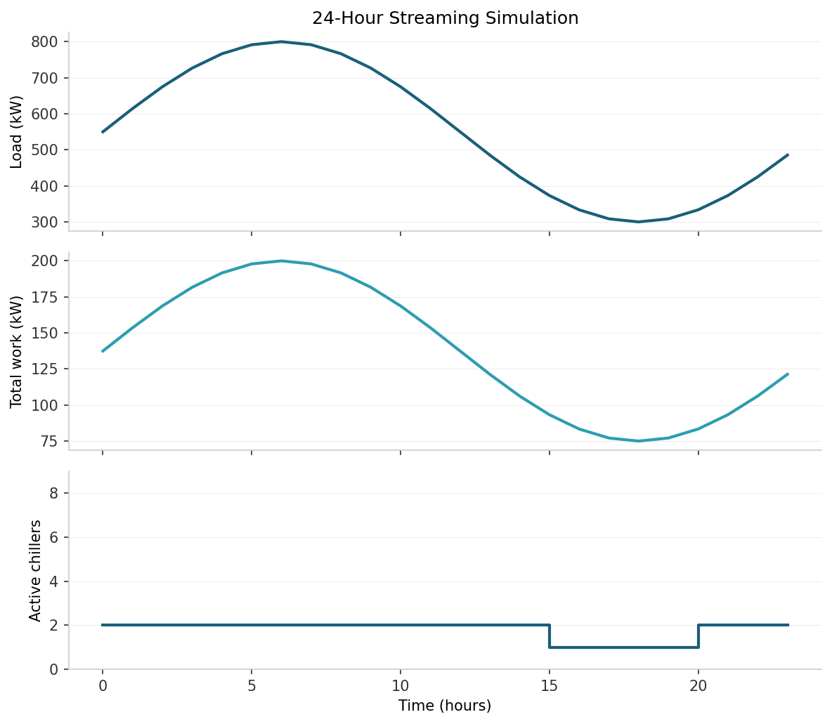
Three-panel line plot sharing the x-axis (time): top = load kW, middle = total work kW, bottom = active chiller count.

Animated chiller grid coloured by COP. Active chillers are coloured on the green–yellow–red scale; inactive chillers are greyed out. The load overlay and savings fraction update each hour as the sinusoidal demand rises and falls.

Example 5 – Time-Varying Wind

Custom wind_fn that rotates wind direction sinusoidally (+-60 deg around 90 deg, 12 h period). Shows total work varying as wind alignment changes.

import math
from chiller_sim import Simulator

def rotating_wind(time_hours: float) -> tuple[float, float]:
    angle = 90.0 + 60.0 * math.sin(2 * math.pi * time_hours / 12)
    return (5.0, angle)

sim = (
    Simulator()
    .with_grid(rows=2, cols=4, spacing_m=10.0, base_cop=4.0, max_cooling_kw=500.0)
    .with_wind_fn(rotating_wind)
    .with_ambient_temp(temp_k=298.15)
    .with_load_fn(lambda t: 1000.0)
    .build()
)

for result in sim.stream(duration_hours=24.0, time_step_hours=1.0):
    angle = 90.0 + 60.0 * math.sin(2 * math.pi * result.time_hours / 12)
    print(f"t={result.time_hours:5.1f}h  angle={angle:6.1f} deg"
          f"  work={result.total_work_kw:7.1f} kW")

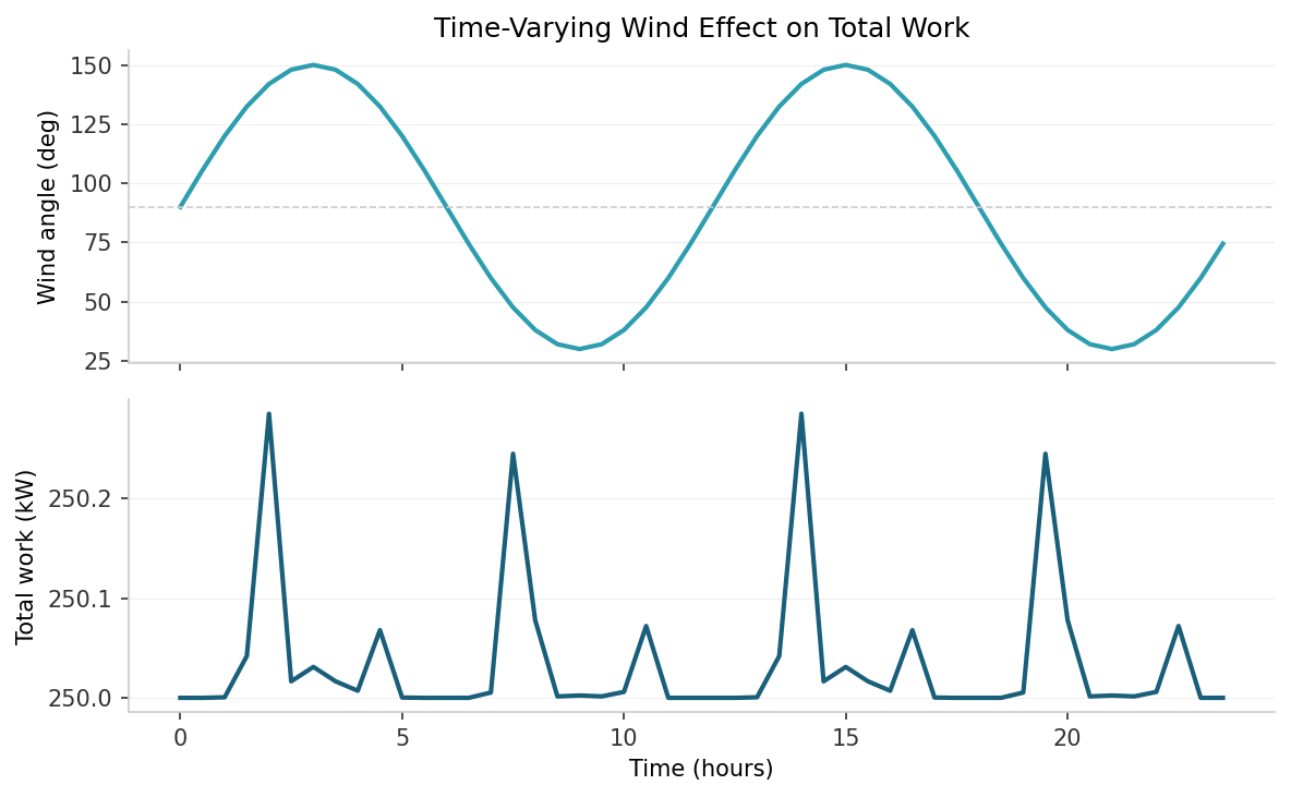
Two-panel line plot – top = wind angle over time, bottom = total work kW over time.

Animated chiller grid coloured by intake temperature rise. The wind vane rotates as the wind direction sweeps +-60 deg around 90 deg, visually showing how chiller-to-chiller thermal interference shifts with wind alignment.